A primer on Graph Neural Networks with Amazon Neptune and the Deep Graph Library
In this post, I’d like to introduce you to Graph Neural Networks (GNN), one of the most exciting developments in Machine Learning (ML) today. Indeed, lots of datasets have an intrinsic graph structure (social networks, fraud detection, cybersecurity, etc.). Flattening them and feeding them to traditional neural network architectures doesn’t feel like the best option. Enter GNNs!
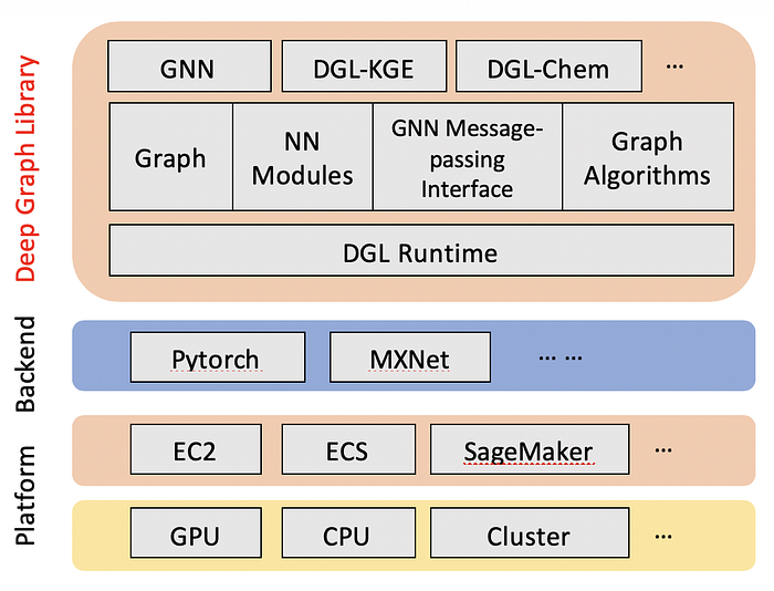
Instead of simply running a sample notebook, let’s throw a few extra ingredients into the mix. In a real life scenario, your graph data would be stored in a graph database, such as Amazon Neptune. You’d pull some data from that database, load it in a notebook, and experiment with an ML library specialized for GNNs, such as the Deep Graph Library. Then, once you’d have figured out which algorithm to use, you’d probably train on the full dataset using a ML service such as Amazon SageMaker.
So how about I show you all of that? Let’s get to
Creating a graph database
Amazon Neptune is a fully managed graph database service.It supports two query languages, Apache TinkerPop Gremlin and W3C’s SPARQL.
Creating a Neptune database is extremely similar to setting up RDS. The simplest way is to use this AWS CloudFormation template. If you want to use the AWS console, the procedure is straightforward.
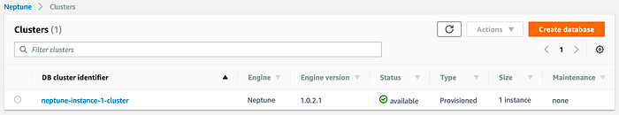
After a few minutes, my Neptune database is up, and we’re ready to load data.
Picking a data set
Let’s use the proverbial Zachary Karate Club data set. It contains 34 vertices and 78 bidirectional edges.
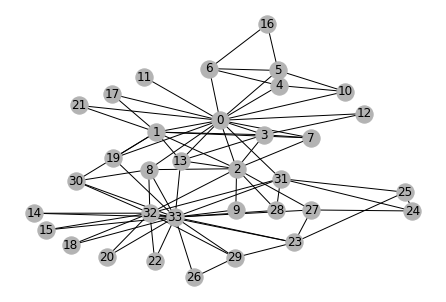
As the story goes, edges represents ties between students and two teachers (nodes 0 and 33). Unfortunately, after an argument between the teachers, the group needs to be split in two. That’s the problem we’re going to solve with a GNN: more on this in a few minutes!
Formatting the data set
Neptune accepts different file formats. I’ll go with the Gremlin format:
- Two CSV files: one for vertices, one for edges.
- Vertex file: id (mandatory), plus a name property (optional).
- Edge file: id, source vertex, destination vertex (all three are mandatory).
Vertex is just a fancy word for node.
Of course, you can (and should) add many more properties in both files.
Here are the two files in Gremlin format.
Loading the data set in Neptune
Neptune is a little peculiar when it comes to loading data:
- A database is only accessible inside og the VPC hosting it. For exemple, you could load data using an EC2 instance or a Lambda function living in that same VPC.
- Neptune requires a VPC Endpoint for S3 in the VPC. This allows Neptune to access S3 directly without using public endpoints. Creating the endpoint takes a few seconds, and you only need to do it once per VPC.
- Data loading is initiated by a curl call. Nothing weird, just pay attention to the parameters.
Ok, with this out of the way, let’s load data. First, I’m copying my two files in an S3 bucket hosted in the same region as my Neptune cluster.
$ aws s3 cp edges.csv s3://jsimon-neptune-useast-1/dgl/
$ aws s3 cp nodes.csv s3://jsimon-neptune-useast-1/dgl/
Then, it’s time for that curl call, using the cluster endpoint visible in the AWS console, or in the output of the CloudFormation template. I’m using the us-east-1 region, you should of course change this if you use a different region.
$ curl -X POST \
 -H ‘Content-Type: application/json’ \
 https://ENDPOINT:PORT/loader -d ‘
 {
 “source” : “s3://jsimon-neptune-useast-1/dgl/”,
 “format” : “csv”,
 “iamRoleArn” : “arn:aws:iam::123456789012:role/NeptuneRoleForS3”,
 “region” : “us-east-1”,
 “failOnError” : “FALSE”,
 “parallelism” : “MEDIUM”,
 “updateSingleCardinalityProperties” : “FALSE”
 }’
If everything is set right, this returns a 200 HTTP status and a job id: I can use it to check if data loading worked ok.
$ curl -G ‘https://ENDPOINT:PORT/loader/8af0f90a-9b72-4835-ab55-2de58918aa81'
{
 “status” : “200 OK”,
 “payload” : {
 “feedCount” : [
 {
 “LOAD_COMPLETED” : 2
 }
 ],
 “overallStatus” : {
   “fullUri” : “s3://jsimon-neptune-useast-1/dgl/”,
   “runNumber” : 1,
   “retryNumber” : 0,
   “status” : “LOAD_COMPLETED”,
   “totalTimeSpent” : 6,
   “startTime” : 1576847947,
   “totalRecords” : 146,
   “totalDuplicates” : 0,
   “parsingErrors” : 0,
   “datatypeMismatchErrors” : 0,
   “insertErrors” : 0
 }
}Things to check (in this order) if you’re having issues: are you in the same VPC? Are you using the correct endpoint and port for Neptune? Is the Security Group for Neptune OK? Is the IAM Role for Neptune OK? Does the S3 Endpoint exist, and does it allow access (endpoint policy) ? Does the S3 bucket exist, and does it allow access (bucket policy)? Do files exist and have the right format? If you still can’t figure it out, the AWS Forum for Neptune is waiting for you ;)
Now let’s connect to Neptune, and explore out data a bit.
Exploring graph data with Gremlin
You can query a Neptune using different languages. I’ll use Python with the gremlinpython library.
$ pip3 install gremlinpython --userConnecting to the Neptune database only requires its endpoint and its port.
Remember that this code must be run inside the appropriate VPC!
Now, I can explore the graph with the Gremlin query language. Here are some examples.
There’s much much more to this, but I’ll stop there. Actually, the only thing that I need to build the graph in my Deep Graph Library script is a list of all edges.
Let’s grab that, and save it to a pickle file.
We’re done with data processing. Let’s now train a GNN!
Training our first GNN with the Deep Graph Library
The Deep Graph Library (DGL) is an open source project that simplifies working with GNN models. It’s implemented in Python, and supports Apache MXNet and PyTorch.
$ pip3 install dgl --userIn the next sections, I’m using a modified version on this tutorial. As usual, the notebook is available on Github.
I also recorded a video where I go through the notebook, and explain every line of code in more detail that you probably care for ;)
Building the graph
First things first: we need to load the list of edges, and build our graph.
Defining the problem
Let’s think about our initial problem for a minute. For each node (student), we want to figure out if it should be grouped with node 0 (the first teacher) or with node 33 (the second teacher).
We can formulate this as a semi-supervised binary classification problem:
- Let’s label node 0 with class 0,
- Let’s label node 33 with class 1,
- All other nodes are unlabeled, and the purpose of the training job will be to learn their correct class.
Building the GNN
Now let’s build the GNN itself. We’ll use a Graph Convolutional Network (GCN), with the following structure:
- Two GCN layers (which we’ll define in a minute). Their purpose is to learn parameters that will help us compute classes for all nodes. In the process, they also gradually shrink the feature space to two dimensions (one for each class).
- A built-in softmax layer, in order to output probabilities for the two classes.
Forward propagation for a GCN layer looks like this:
- Set input features for all nodes,
- Ask each node to send its features across all its edges,
- At each destination node, update features to the sum of source node features (this is the secret sauce in GCNs),
- Apply a linear transformation (think Y=WX+B… with matrices) to reduce dimensionality.
As you can see in the code below, DGL provides simple message passing semantics to handle node communication.
Let me repeat the central idea in GCNs: the features of each node will be repeatedly updated by summing the features of adjacent nodes. This is similar to the convolution operation implemented in Convolution Neural Networks (which sums adjacent pixel values), hence the GCN name.
Why this works is beyond the scope of this post. If you’re curious about GCN theory, this excellent 2-part post is the best I’ve found. Of course, you can also read the research paper.
Training the GNN
Input features are stored in a matrix (number_of_nodes lines and number_of_features columns).
Here, the only feature for each node is a one-hot encoded vector representing the node id. Stacking all node vectors, we get an identity matrix of size node_count, which we can easily build with torch.eye().
DGL makes it easy to assign node features. In the code above, g.ndata[‘h’] = inputs creates a feature named ‘h’ on each node, and sets it to the appropriate row in the inputs matrix.
In a real-life scenario, we would use more features, probably extracted or computed from the graph database, e.g. node properties, distance to nodes 0 and 33, etc.
We also need to define labels: we only label nodes 0 and 33, respectively with class 0 and 1.
The training loop itself is PyTorch business as usual:
- Run forward propagation on the graph and its inputs,
- Compute the loss between predictions and labels (only for labeled nodes),
- Run backpropagation, and update layer weights.
Let’s try to put this in plain English: by learning from two labeled nodes, we update layer parameters that let us compute class probabilities for all other nodes.
Visualizing results
Once training is complete, we can easily find the class of all nodes by looking at the epoch outputs.
A picture is worth a thousand words!
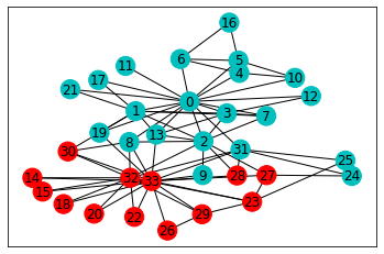


Pretty cool! This looks like a reasonable split, doesn’t it?
Training at scale with Amazon SageMaker
DGL is available in the AWS Deep Learning Containers, which you can easily train on EC2, container services, and of course on Amazon SageMaker.
If you’d like to know more about combining DGL and SageMaker, here are some resources:
- Blog post,
- AWS documentation,
- Sample notebooks.
Conclusion
That’s it for today. I hope you now have a basic understanding of GNNs, and how to get started with them on AWS.
As always, thank you for reading. Happy to answer questions here or on Twitter.